Temporal difference learning is one of the reinforcement learning methods and is a value-based method.
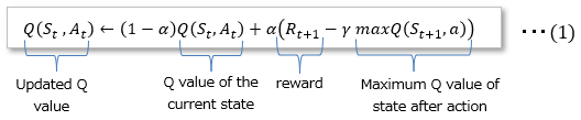
The Q value is determined using the action value function that makes the TD error 0 as shown in formula (1) below.
Reinforcement learning is explained here. This page explains using a simple Skinner box to understand the implementation example of TD learning.
■Examples of TD learning
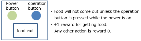
Here is a Skinner box that looks like this: There is a power button and an operation button, and the mouse can take out food by pressing the operation button while the power is on. Replacing this with TD learning, +1 reward if you can take out the food.
No food is given for other actions, and the reward is 0.
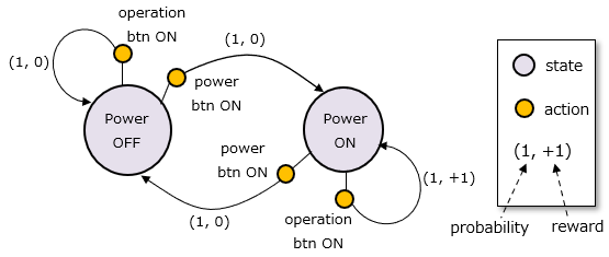
The mouse's behavior, reward, and power supply state are expressed in a state transition diagram according to the Markov Decision Process.
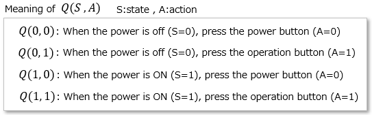
<Q value:indicators for action>
In order for the mouse to receive the reward, it is good to press the operation button when the power is on, and it is good to turn the power on when the power is off.
The action that should be taken in each state is expressed by the Q value. And reinforcement learning is to learn this Q value.
The Q value is expressed as follows, and each state and action pattern has a value, and the largest value in each state is the action that should be taken.
The Q value in TD learning can be calculated from the Bellman equation as follows. The arrow (←) has the same meaning as the equal (=).
For example, in this example, it is only after the mouse receives a reward that it can be evaluated whether its actions have been correct so far, so you might think that the Q value can be updated at the end of the test.
You can update the Q value to , and let it update the Q value of the state resulting from the action based on the Q value of the current state.
This formula is synonymous with exponentially averaging the current Q value and future Q value with α.
γ is a reflection coefficient for the Q value, which is a discount rate derived from uncertain factors for the future.
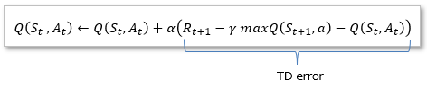
Equation (1) changes as follows, and the following part is called TD error. We need to learn the action-value function so that this TD error is 0.
<Calculate the Q value>
Specifically calculate the Q value in the above example.
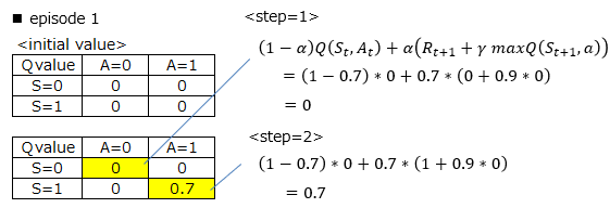
The initial Q values are all 0 in any state. Initially, the state is set to 0 (power off).
Here, the action with the largest Q value at state 0 is selected, but since all Q values are equal, the action is selected at random.
This time, action 0 (power button ON) was selected.
At this time, the Q value is updated according to the result of the action, but since the reward cannot be obtained at this point, the calculation result of (1) is 0.
The next action is also chosen randomly because the Q value is equal. Here, state 1 (power ON) and action 1 (operation button ON) were selected.
Then I got a reward, so the calculation result of (1) was 0.7 and I was able to update the Q value. This is the end of one episode
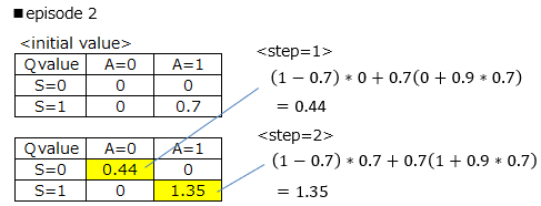
Then start the episode from the beginning again. The initial value is the final Q value of the previous episode.
The action with the maximum Q value when the state is 0 is 0, so we choose this. At this time, the Q value of the state after taking action has a value, so you cannot get a reward, but you can update the Q value.
Next, select the maximum Q value in the same way as in state 1.
The action becomes 1, and the Q value is updated in the same way.
<Finding the optimal Q value by the ε-greedy method>
If you select the action with the largest Q value as above, that action may always be selected once the value is updated.
There may well be better choices out there. To prevent this, one of the methods is called the ε-greedy method, in which actions are randomly selected at the beginning of the episode, and actions are selected by relying on the Q value as the episode progresses.
The python implementation part of the next section is as follows.
The number of episodes is 10, and the number of trials per episode is 4. As a result, the Q value is as follows.
The result is that it is better to turn the power button ON (S=0, A=0) when the power is OFF, and turn the operation button ON (S=1, A=1) when the power is ON. That's right.
[[5.69584585 0.1974375 ]
[0.47434359 7.36479906]]
■Q-value learning methods other than TD learning
<Monte Carlo method>
While TD learning is to update the Q value sequentially, Monte Carlo method is to update the Q value at the end of the episode.
The Monte Carlo method has the advantage of high accuracy of the Q value because the Q value is updated based on the results of the episode, but the disadvantage is that online learning is difficult because the update is slow.
An implementation example of the Monte Carlo method is here.