How to draw a Bode plot(secondary delay system)

・In Japanese

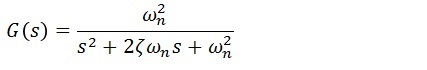
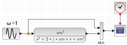
I will explain how to draw a Bode diagram of the transfer function of the second-order lag system. Click here for the basics of how to draw a Bode plot.


(ω = natural frequency , ζ = Attenuation coefficient)

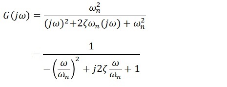
Substitute "s = jω" into the above equation and transform the equation as follows.


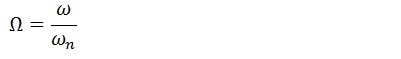
here

and

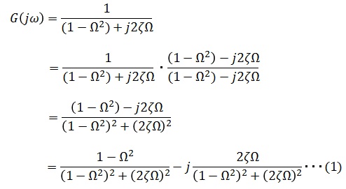
■Represented on the complex plane
Eq. (1) is expressed on the complex plane as follows. In order to draw a Bode plot, it is necessary to find the absolute value and angle of G (jω).



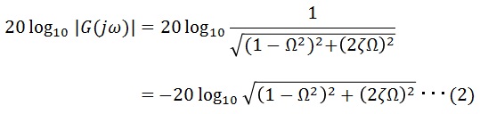
■Gain characteristics
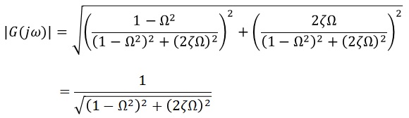
The absolute value of G (jΩ) is as follows.



From the decibel calculation method, it is as follows.




Since the above characteristics change depending on the value of Ω, we will classify the cases.

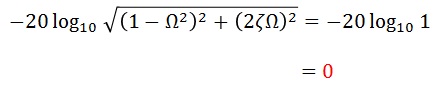
■When Ω << 1 (sufficiently smaller than 1)
From equation (2),



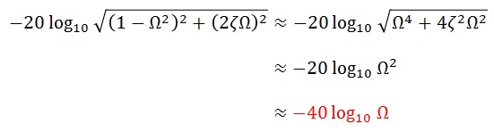
■When Ω >> 1 (sufficiently larger than 1)
From equation (2),


■When Ω = 1
From equation (2),


Here, the characteristics change depending on the value of ζ, so we will further classify the cases.

　　・ When 2ζ> 1
　　

　　・When 0 < 2ζ< 1
　　

＜Bode plot＞
From the above, the Bode plot is as follows.



■Phase characteristics
The phase characteristics are easy to understand when considered on the complex plane. Since the characteristics of this also change depending on the value of ω, we will classify the cases.

■When Ω << 1 (sufficiently smaller than 1)
Since the imaginary component is 0 and is on the real axis, the phase is 0 degrees.



■When Ω=1
Since the real component is 0 and it is on the imaginary axis, the phase is -90 degrees.



■When Ω >> 1 (sufficiently larger than 1)
The real component is 1 / Ω² and the imaginary component is 1 / Ω³. As Ω increases, the imaginary component becomes smaller and closer to the real axis, so the phase approaches -180 degrees.



＜Bode plot＞
From the above, the Bode plot is as follows. The detailed explanation is omitted, but the characteristics also change depending on the value of ζ. However, no matter what the value of ζ, when Ω = 1, the phase is delayed by 90 degrees.



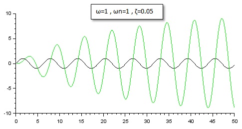
■simulation result
When ω=1 , ωn=1 , ζ=0.05, that is, when there is a gain on the board diagram, the simulation results are as follows. You can see that the output (green line) becomes larger and larger in relation to the input (black line), and diverges. This frequency is called the resonance frequency. (Click here to see how to use Scilab)

List of related articles TOP MENU Control theory Transfer function Transfer function Transfer function synthesis Closed/Open-loop transfer function Analog filter Low Pass Filter ・First-order delay system 　・Transfer function 　・Bode plot ・secondary delay system 　・Bode plot ・Butterworth filter ・Bessel filter All pass filter 　・Transfer function 　・Pade approximation Notch filter Band pass filter