Pade approximation

　・In Japanese
＜Premise knowledge＞
　・How to draw a Bode plot
　・Scilab
　・Dead-time transfer function

■What is Pade approximation?

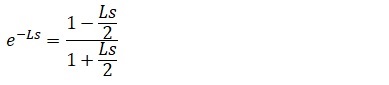
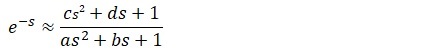
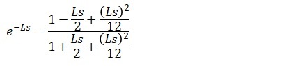
Pade approximation is one of the methods of approximating functions. For example, the dead time can be expressed by the following transfer function, but it cannot be used as it is because it has nonlinear characteristics, and it must be linearly approximated. Therefore, the Padé approximation can be used for linear approximation.



The Pade approximation function is:

＜First-order Padé approximation＞

　

A better approximation can be achieved using the second-order Padé approximation.

＜Second-order Padé approximation＞

　

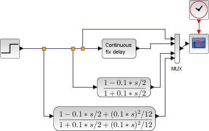
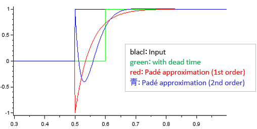
■Observe the Padé approximation in action

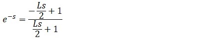
Observe the Padé approximation in action. The design result in Scilab is as follows. Here, the dead time is set to 0.1 seconds.


The simulation results are as follows. The Padé approximation has the characteristic that the value drops once, but this is in a form that approaches the rise timing of the dead time.

■How to derive the Padé approximation

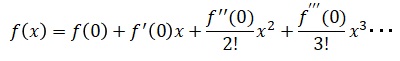
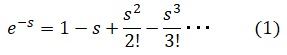
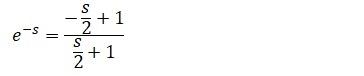
For simplicity, consider the e^-s approximation. First, the Maclaurin expansion is as follows.



Therefore,


This is an approximation, but it is difficult to handle, so I express it with the following advantageous function.



Maclaurin expansion of the above equation gives (Click here for the derivation method) :



Comparing (1) and (2), we get

Than,


Since this solution does not satisfy the following equation for the third-order part, it is an approximation up to the second-order.



Therefore, it is as follows.



Since s = Ls here, the following is obtained, and the first-order Padé approximation is derived.



Similarly, when deriving the second-order Padé approximation, put the following, Maclaurin expansion, and compare with Eq. (1).

List of related articles TOP MENU Control theory Transfer function Transfer function Transfer function synthesis Closed/Open-loop transfer function Analog filter Low Pass Filter ・First-order delay system 　・Transfer function 　・Bode plot ・secondary delay system 　・Bode plot ・Butterworth filter ・Bessel filter All pass filter 　・Transfer function 　・Pade approximation Notch filter Band pass filter